
Understand and Use Quartiles, Control Limits and Natural Process Limits to Optimize Your Flow Performance
As part of process management, performance monitoring is essential to ensure stability and efficiency.
To do this, different statistical methods exist to analyze variations in workflows and identify significant gaps.
Some of the most commonly used tools include Quartiles, Control Limits (UCL/LCL), and Natural Process Limits (UNPL/LNPL).
But what do these barbaric terms mean?
This article aims to demystify these concepts and explain how and when to use them to optimize your processes.
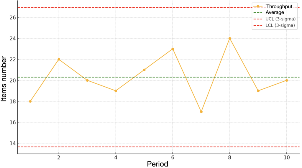
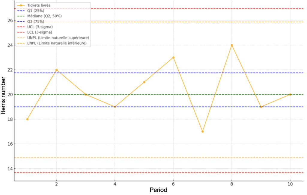
But before going into the details of each concept, it would be relevant to start the article with an illustrative graph that shows the number of tickets delivered over time periods (like in the example we used). This will serve as the basis for the explanations to come.
Example data: Number of tickets delivered by a team over 10 two-week periods: 18; 22; 20; 19; 21; 23; 17; 24; 19; 20
Quartiles: Analyze the Distribution of the Performance of Your Flow Time
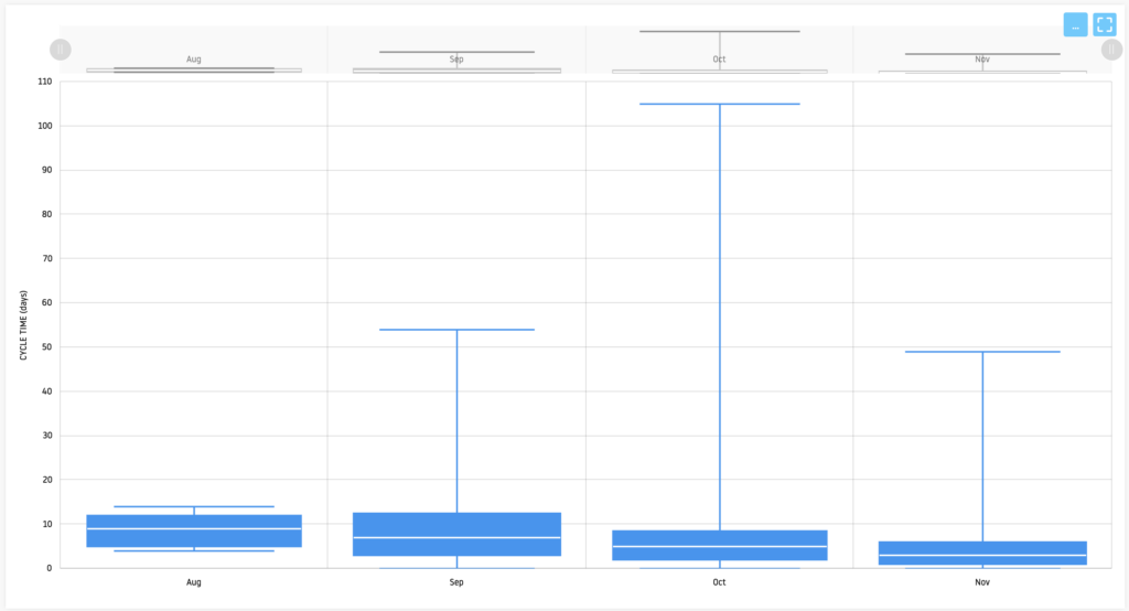
Quartiles – also called whisker boxes – divide the data into four equal parts, allowing us to understand how they are distributed.
They are particularly useful for getting an overview of the performance distribution in a process.
Definition of Quartiles
- Q1 (First quartile): 25% of data is below this value.
- Q2 (Median or second quartile): 50% of the data is lower than this value.
- Q3 (Third quartile): 75% of data is below this value.
Inter-quartile ranges (IQR) can also be used to detect outliers.
The IQR will represent the lower and upper limits admissible to have a predictable flow distribution. These are the famous mustaches. Values falling outside must be considered as outliers and analyzed.
The IQR is defined as Q3−Q1.
A common rule is to consider any value outside of Q1 − 1.5 × IQR and Q3 + 1.5 × IQR as an outlier.
Example of calculating Quartiles
- Sort data in ascending order: 17; 18; 19; 19; 20; 20; 21; 22; 23; 24
- Calculate the First Quartile – Q1 by identifying the Cycle time of 25% of the measurements – Result: Q1 = 19
- Calculate the Second Quartile, i.e. the Median, representing 50% of the measured cycle times – Result Q2 = 20
- Odd List: When the number of measures is odd, take the middle value
- Even List: When the number of measurements is even, as in our example, add the 2 central values and divide them by 2. The result represents the Median.
- Calculate the Third Quartile – Q3, representing 75% of measurements taken – Result: Q3 = 22
- Calculate the inter-quartile (IQR)
- IQR = Q3 – Q1 = 22 – 19 = 3
- Low limit = Q1 – 1.5*IQR = 19 + 1.5*3 = 14.5
- High limit = Q3 + 1.5*IQR = 22 + 15*3 = 26.5

Why use quartiles?
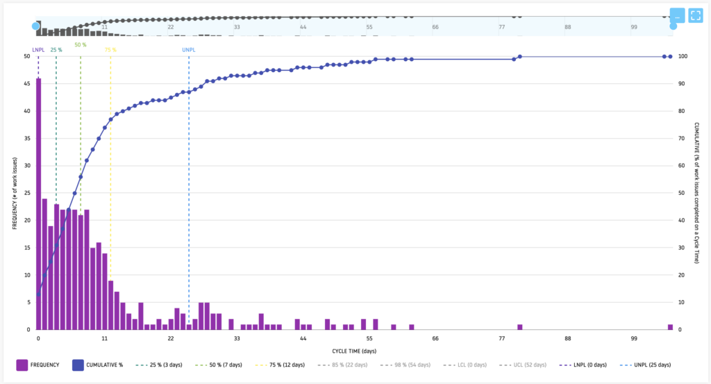
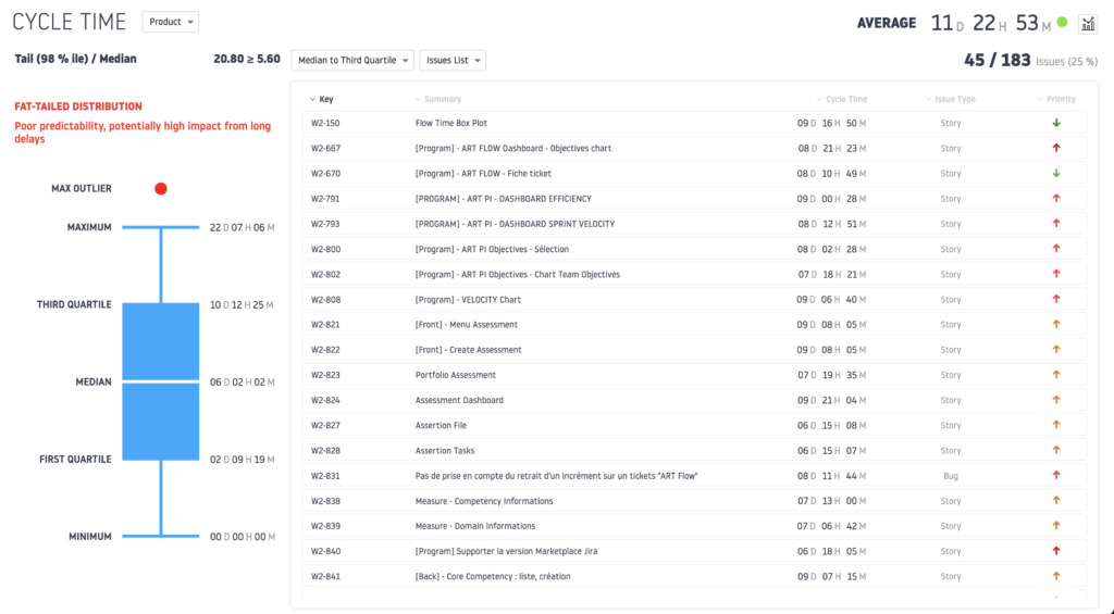
Quartiles are often used to visualize the distribution of data and identify points where the majority of values fall. This allows you to see where the central values are (using the median) and identify gaps or outliers.
Let’s take the example of a development team that delivers tickets every two weeks. By analyzing the number of tickets delivered over multiple periods, quartiles give us insight into the distribution of deliveries. This helps understand how many tickets are delivered in the bottom 25%, middle 50%, and top 25%.
Example of using Quartiles on Wiveez
UCL/LCL: Keeping your Process under Control
Control limits (UCL and LCL) are statistical thresholds used in control charts. They allow a process to be monitored to detect anomalies and determine whether it is stable.
- UCL (Upper Control Limit): Upper control limit.
- LCL (Lower Control Limit): Lower control limit. These limits are typically set at 3 standard deviations above and below the mean, meaning that 99.73% of the data should fall within this range in an “in control” process.
Why use Control Limit?
Control limits are ideal for detecting anomalies in a process. If any data falls outside of these limits, it may indicate a problem that requires investigation (such as an unexpected change in performance).
UCL/LCL: How to calculate them?
Control limits (UCL/LCL) are used in control charts to monitor a process. They are based on the mean and standard deviation, and define a normal range of variation. They are calculated by applying the 3-sigma rule, i.e. three standard deviations above and below the average.
Calculation steps:
1 – Calculate the average:

2 – Calculate standard deviation:

3 – Calculate Control Limits (LCL & UCL):

UNPL/LNPL: Understanding Natural Variability
Unlike UCL and LCL, Natural Process Limits (UNPL and LNPL) are not based solely on statistical calculations, but rather on a thorough understanding of the process and accepted tolerances.
- UNPL (Upper Natural Process Limit): Natural upper limit.
- LNPL (Lower Natural Process Limit): Natural lower limit. These limits reflect the natural range of variation of the process, defined by accepted specifications or tolerances, not by statistical deviations alone.
Why use Natural Process Limits?
Natural limits are particularly useful when you have a good empirical understanding of the process or when specific tolerances must be met (for example, industry standards or customer requirements). They help avoid overreacting to small variations while ensuring that the process operates within the defined acceptable range.
Example
- Data collection and distribution analysis
- In general, the first step is to identify whether the process follows a normal distribution or not. Natural boundaries can sometimes be calculated differently depending on the distribution of the data.
- Determine acceptable tolerances
- UNPL/LNPL can be based on accepted tolerances or performance specifications defined by business needs, customer requirements or internal standards. If these tolerances exist (for example, a team expects to deliver between 15 and 25 tickets per iteration), they can directly guide the calculations.
- If specifications or tolerances are already established, natural limits can be set accordingly. For example, if the team considers that by delivering less than 16 tickets or more than 26, it is departing from its normal behavior, then:
- LNPL = 16
- UNPL = 26
- Calculate natural limits based on observed variability
- If you do not have pre-established tolerances, you can calculate UNPL/LNPL based on historical process data.
- Calculate the median or an adjusted average
- The median is often used instead of the mean if the process has outliers or asymmetric variations. This gives a central measurement less influenced by extreme values.
- In our case, the median of tickets delivered over 10 periods is:
- Median = 20
- If you use the average, it is: Average(xˉ) = 20.3
- Calculate the natural range of variability
- The natural variability of the process is often estimated from the interquartile range (IQR), which measures the dispersion between the lowest 25% of data and the highest 25%.
- For our example, the quartiles are as follows:
- Q1 (1st quartile)=19: 25% of tickets delivered are less than or equal to 19.
- Q3(3rd quartile)=22: 75% of tickets delivered are less than or equal to 22.
- The interquartile range (IQR) is: IQR = Q3−Q1 = 22−19 = 3
- Calculate natural limits
- A common method is to multiply the IQR by a factor, often 1.5×IQR, to identify the acceptable range of variation.
- Thus, the natural limits can be calculated as follows:
- UNPL = Q3+1.5×IQR = 22+1.5×3 =22+4.5 = 26.5
- LNPL= Q1−1.5×IQR = 19−1.5×3 = 19−4.5 = 14.5
- Adjust limits based on observations and specifications
- Once the initial limits are calculated, you can adjust them based on empirical observations or process goals.
- For example, if your team finds that delivering fewer than 16 tickets or more than 26 tickets is unacceptable, you could set the UNPL/LNPL respectively to those values, even if the calculations indicate a slight variation.
You see, based on this example, that the UNPL and the LNPL are very complementary to the measurement with the Quartiles by integrating the limits not to be exceeded to remain in a stable system.
Comparison of UNPL/LNPL calculations with UCL/LCL
Returning to our example with delivered tickets:
- Calculation of UCL/LCL (based on 3-sigma):
- UCL = xˉ+3σ = 20.3+3×2.33 = 27.29
- LCL = xˉ−3σ = 20.3−3×2.33 = 13.31
- Calculation of UNPL/LNPL (based on 1.5 x IQR):
- UNPL = 26.5
- LNPL = 14.5
The natural limits (UNPL/LNPL) are therefore a little tighter than the UCL/LCL control limits, in this example.
This shows that the UNPL/LNPL reflects the natural variation of the process (based on quartiles) more than the control limits, which are based only on the mean and standard deviation.
UNPL and LNPL are calculated based on natural variability and empirical understanding of the process, often with measures like quartiles or IQR.
Unlike UCL and LCL, natural limits are not only intended to detect statistical anomalies, but to define the expected performance limits of a process based on its natural capacity or external specifications.
When to Use Quartiles, UCL/LCL, and UNPL/LNPL?
Understanding quartiles, control limits (UCL/LCL) and natural limits (UNPL/LNPL) is essential for effective process management. Here’s how and when to use them:
- Quartiles: Use them to get an overview of data distribution and identify general trends in process performance. They are particularly useful for descriptive statistical analyses.
- UCL/LCL: Use control limits when you want to monitor the statistical stability of your process and detect anomalies that require immediate intervention.
- UNPL/LNPL: Use natural limits when you need to set specific tolerances (based on standards or requirements) and want to capture the natural variability of a process without overreacting to small variations.
Conclusion
Understanding the difference between quartiles, UCL/LCL and UNPL/LNPL is essential to successfully manage process performance.
Each of these methods brings a different perspective, ranging from data distribution to statistical monitoring to the management of natural tolerances.
By learning how to use these tools properly, you can improve the stability of your processes, avoid false alarms and maximize efficiency.
Whether you are looking to monitor the performance of a project team or optimize a manufacturing process, these concepts will help you make better decisions to keep your processes under control.


